第二步:模型训练
在本教程中,我们将演示如何训练一个GLUE模型来集成未配对的单个细胞多基因组数据。我们继续上一个scRNA-seq和scATAC-seq数据集的教程。
[1]:
from itertools import chain

import anndata as ad
import itertools
import networkx as nx
import pandas as pd
import scanpy as sc
import scglue
import seaborn as sns
from matplotlib import rcParams
[2]:
scglue.plot.set_publication_params()
rcParams["figure.figsize"] = (4, 4)
读取预处理数据
首先,读取 第一步 预处理过的数据。
[3]:
rna = ad.read_h5ad("rna-pp.h5ad")
atac = ad.read_h5ad("atac-pp.h5ad")
guidance = nx.read_graphml("guidance.graphml.gz")
配置数据
(预计时间:忽略不计)
在模型训练之前,我们需要使用 scglue.models.configure_dataset 来配置数据集。对于要整合的数据集,需要指定使用的概率生成模型。这里我们使用负二项分布 NB 对scRNA-seq和scATAC-seq的原始计数进行建模。
可选的,我们可以指定是否只使用高度可变的特征(use_highly_variable),使用哪个数据层(use_layer),以及哪个预处理嵌入(use_rep)作为编码器的第一个转换。
For the scRNA-seq data, we use the previously backed up raw counts in the “counts” layer, and use the PCA embedding as the first encoder transformation.
For the scATAC-seq data, the raw counts are just
atac.X, so it’s unnecessary to specifyuse_layer. We use the LSI embedding as the first encoder transformation.
[4]:
scglue.models.configure_dataset(
    rna, "NB", use_highly_variable=True,
    use_layer="counts", use_rep="X_pca"
)
[5]:
scglue.models.configure_dataset(
    atac, "NB", use_highly_variable=True,
    use_rep="X_lsi"
)
scglue.models.configure_dataset 的其他有用选项包括:
use_batch:将其设置为“obs”中的一列,可以告诉模型将它作为批次效应进行校正;use_cell_type:将其设置为“obs”中的一列,可以告诉模型将它作为细胞类型标签进行有监督学习。
接着,由于我们只使用高度可变的特征,我们也从完整引导图中提取只包含高度可变的特征的子图:
[6]:
guidance_hvf = guidance.subgraph(chain(
    rna.var.query("highly_variable").index,
    atac.var.query("highly_variable").index
)).copy()
训练GLUE模型
(预计时间:15-60分钟,取决于计算设备)
接着,训练 GLUE模型 整合两个组学层。
要整合的数据集被指定为
dict,键是模态名,模态名由您决定,只要它们保持一致(见下)。我们为fit函数指定了一个目录,模型快照和训练日志都将被储存在这里。
对于更高级的用法,请参考 函数文档。
[7]:
glue = scglue.models.fit_SCGLUE(
    {"rna": rna, "atac": atac}, guidance_hvf,
    fit_kws={"directory": "glue"}
)
[INFO] fit_SCGLUE: Pretraining SCGLUE model...
[INFO] autodevice: Using GPU 0 as computation device.
[INFO] check_graph: Checking variable coverage...
[INFO] check_graph: Checking edge attributes...
[INFO] check_graph: Checking self-loops...
[INFO] check_graph: Checking graph symmetry...
[INFO] SCGLUEModel: Setting `graph_batch_size` = 27025
[INFO] SCGLUEModel: Setting `max_epochs` = 186
[INFO] SCGLUEModel: Setting `patience` = 16
[INFO] SCGLUEModel: Setting `reduce_lr_patience` = 8
[INFO] SCGLUETrainer: Using training directory: "glue/pretrain"
[INFO] SCGLUETrainer: [Epoch 10] train={'g_nll': 0.451, 'g_kl': 0.004, 'g_elbo': 0.456, 'x_rna_nll': 0.165, 'x_rna_kl': 0.006, 'x_rna_elbo': 0.171, 'x_atac_nll': 0.04, 'x_atac_kl': 0.0, 'x_atac_elbo': 0.041, 'dsc_loss': 0.692, 'vae_loss': 0.23, 'gen_loss': 0.196}, val={'g_nll': 0.45, 'g_kl': 0.004, 'g_elbo': 0.454, 'x_rna_nll': 0.166, 'x_rna_kl': 0.006, 'x_rna_elbo': 0.172, 'x_atac_nll': 0.04, 'x_atac_kl': 0.0, 'x_atac_elbo': 0.04, 'dsc_loss': 0.694, 'vae_loss': 0.23, 'gen_loss': 0.195}, 6.1s elapsed
[INFO] SCGLUETrainer: [Epoch 20] train={'g_nll': 0.432, 'g_kl': 0.004, 'g_elbo': 0.436, 'x_rna_nll': 0.163, 'x_rna_kl': 0.006, 'x_rna_elbo': 0.17, 'x_atac_nll': 0.04, 'x_atac_kl': 0.0, 'x_atac_elbo': 0.04, 'dsc_loss': 0.693, 'vae_loss': 0.227, 'gen_loss': 0.192}, val={'g_nll': 0.432, 'g_kl': 0.004, 'g_elbo': 0.436, 'x_rna_nll': 0.163, 'x_rna_kl': 0.006, 'x_rna_elbo': 0.169, 'x_atac_nll': 0.04, 'x_atac_kl': 0.0, 'x_atac_elbo': 0.04, 'dsc_loss': 0.695, 'vae_loss': 0.227, 'gen_loss': 0.192}, 6.1s elapsed
[INFO] SCGLUETrainer: [Epoch 30] train={'g_nll': 0.424, 'g_kl': 0.004, 'g_elbo': 0.428, 'x_rna_nll': 0.162, 'x_rna_kl': 0.006, 'x_rna_elbo': 0.168, 'x_atac_nll': 0.04, 'x_atac_kl': 0.0, 'x_atac_elbo': 0.04, 'dsc_loss': 0.693, 'vae_loss': 0.225, 'gen_loss': 0.19}, val={'g_nll': 0.424, 'g_kl': 0.004, 'g_elbo': 0.427, 'x_rna_nll': 0.165, 'x_rna_kl': 0.006, 'x_rna_elbo': 0.171, 'x_atac_nll': 0.04, 'x_atac_kl': 0.0, 'x_atac_elbo': 0.04, 'dsc_loss': 0.694, 'vae_loss': 0.228, 'gen_loss': 0.193}, 6.4s elapsed
Epoch 00034: reducing learning rate of group 0 to 2.0000e-04.
Epoch 00034: reducing learning rate of group 0 to 2.0000e-04.
[INFO] LRScheduler: Learning rate reduction: step 1
[INFO] SCGLUETrainer: [Epoch 40] train={'g_nll': 0.42, 'g_kl': 0.004, 'g_elbo': 0.424, 'x_rna_nll': 0.161, 'x_rna_kl': 0.006, 'x_rna_elbo': 0.167, 'x_atac_nll': 0.039, 'x_atac_kl': 0.0, 'x_atac_elbo': 0.04, 'dsc_loss': 0.693, 'vae_loss': 0.224, 'gen_loss': 0.189}, val={'g_nll': 0.42, 'g_kl': 0.004, 'g_elbo': 0.423, 'x_rna_nll': 0.163, 'x_rna_kl': 0.006, 'x_rna_elbo': 0.169, 'x_atac_nll': 0.04, 'x_atac_kl': 0.0, 'x_atac_elbo': 0.04, 'dsc_loss': 0.693, 'vae_loss': 0.226, 'gen_loss': 0.191}, 5.7s elapsed
Epoch 00045: reducing learning rate of group 0 to 2.0000e-05.
Epoch 00045: reducing learning rate of group 0 to 2.0000e-05.
[INFO] LRScheduler: Learning rate reduction: step 2
[INFO] SCGLUETrainer: [Epoch 50] train={'g_nll': 0.42, 'g_kl': 0.004, 'g_elbo': 0.424, 'x_rna_nll': 0.161, 'x_rna_kl': 0.006, 'x_rna_elbo': 0.167, 'x_atac_nll': 0.039, 'x_atac_kl': 0.0, 'x_atac_elbo': 0.04, 'dsc_loss': 0.693, 'vae_loss': 0.223, 'gen_loss': 0.189}, val={'g_nll': 0.421, 'g_kl': 0.004, 'g_elbo': 0.424, 'x_rna_nll': 0.161, 'x_rna_kl': 0.006, 'x_rna_elbo': 0.167, 'x_atac_nll': 0.04, 'x_atac_kl': 0.0, 'x_atac_elbo': 0.04, 'dsc_loss': 0.693, 'vae_loss': 0.224, 'gen_loss': 0.189}, 5.9s elapsed
2022-08-10 11:15:59,205 ignite.handlers.early_stopping.EarlyStopping INFO: EarlyStopping: Stop training
[INFO] EarlyStopping: Restoring checkpoint "52"...
[INFO] fit_SCGLUE: Estimating balancing weight...
[INFO] estimate_balancing_weight: Clustering cells...
[INFO] estimate_balancing_weight: Matching clusters...
[INFO] estimate_balancing_weight: Matching array shape = (16, 18)...
[INFO] estimate_balancing_weight: Estimating balancing weight...
[INFO] fit_SCGLUE: Fine-tuning SCGLUE model...
[INFO] check_graph: Checking variable coverage...
[INFO] check_graph: Checking edge attributes...
[INFO] check_graph: Checking self-loops...
[INFO] check_graph: Checking graph symmetry...
[INFO] SCGLUEModel: Setting `graph_batch_size` = 27025
[INFO] SCGLUEModel: Setting `align_burnin` = 31
[INFO] SCGLUEModel: Setting `max_epochs` = 186
[INFO] SCGLUEModel: Setting `patience` = 16
[INFO] SCGLUEModel: Setting `reduce_lr_patience` = 8
[INFO] SCGLUETrainer: Using training directory: "glue/fine-tune"
[INFO] SCGLUETrainer: [Epoch 10] train={'g_nll': 0.418, 'g_kl': 0.004, 'g_elbo': 0.421, 'x_rna_nll': 0.161, 'x_rna_kl': 0.006, 'x_rna_elbo': 0.167, 'x_atac_nll': 0.039, 'x_atac_kl': 0.0, 'x_atac_elbo': 0.04, 'dsc_loss': 0.691, 'vae_loss': 0.223, 'gen_loss': 0.189}, val={'g_nll': 0.416, 'g_kl': 0.004, 'g_elbo': 0.42, 'x_rna_nll': 0.167, 'x_rna_kl': 0.006, 'x_rna_elbo': 0.173, 'x_atac_nll': 0.04, 'x_atac_kl': 0.0, 'x_atac_elbo': 0.04, 'dsc_loss': 0.68, 'vae_loss': 0.229, 'gen_loss': 0.195}, 7.0s elapsed
[INFO] SCGLUETrainer: [Epoch 20] train={'g_nll': 0.415, 'g_kl': 0.004, 'g_elbo': 0.418, 'x_rna_nll': 0.161, 'x_rna_kl': 0.005, 'x_rna_elbo': 0.166, 'x_atac_nll': 0.039, 'x_atac_kl': 0.0, 'x_atac_elbo': 0.04, 'dsc_loss': 0.694, 'vae_loss': 0.223, 'gen_loss': 0.188}, val={'g_nll': 0.415, 'g_kl': 0.003, 'g_elbo': 0.418, 'x_rna_nll': 0.168, 'x_rna_kl': 0.005, 'x_rna_elbo': 0.174, 'x_atac_nll': 0.039, 'x_atac_kl': 0.0, 'x_atac_elbo': 0.04, 'dsc_loss': 0.684, 'vae_loss': 0.23, 'gen_loss': 0.196}, 8.3s elapsed
[INFO] SCGLUETrainer: [Epoch 30] train={'g_nll': 0.413, 'g_kl': 0.003, 'g_elbo': 0.416, 'x_rna_nll': 0.16, 'x_rna_kl': 0.005, 'x_rna_elbo': 0.166, 'x_atac_nll': 0.039, 'x_atac_kl': 0.0, 'x_atac_elbo': 0.04, 'dsc_loss': 0.694, 'vae_loss': 0.222, 'gen_loss': 0.187}, val={'g_nll': 0.412, 'g_kl': 0.003, 'g_elbo': 0.416, 'x_rna_nll': 0.168, 'x_rna_kl': 0.005, 'x_rna_elbo': 0.173, 'x_atac_nll': 0.04, 'x_atac_kl': 0.0, 'x_atac_elbo': 0.04, 'dsc_loss': 0.675, 'vae_loss': 0.23, 'gen_loss': 0.196}, 8.4s elapsed
[INFO] SCGLUETrainer: [Epoch 40] train={'g_nll': 0.411, 'g_kl': 0.003, 'g_elbo': 0.415, 'x_rna_nll': 0.161, 'x_rna_kl': 0.005, 'x_rna_elbo': 0.166, 'x_atac_nll': 0.039, 'x_atac_kl': 0.0, 'x_atac_elbo': 0.039, 'dsc_loss': 0.692, 'vae_loss': 0.222, 'gen_loss': 0.188}, val={'g_nll': 0.411, 'g_kl': 0.003, 'g_elbo': 0.414, 'x_rna_nll': 0.167, 'x_rna_kl': 0.005, 'x_rna_elbo': 0.172, 'x_atac_nll': 0.039, 'x_atac_kl': 0.0, 'x_atac_elbo': 0.04, 'dsc_loss': 0.675, 'vae_loss': 0.229, 'gen_loss': 0.195}, 6.6s elapsed
[INFO] SCGLUETrainer: [Epoch 50] train={'g_nll': 0.411, 'g_kl': 0.003, 'g_elbo': 0.414, 'x_rna_nll': 0.16, 'x_rna_kl': 0.005, 'x_rna_elbo': 0.165, 'x_atac_nll': 0.039, 'x_atac_kl': 0.0, 'x_atac_elbo': 0.039, 'dsc_loss': 0.692, 'vae_loss': 0.221, 'gen_loss': 0.187}, val={'g_nll': 0.411, 'g_kl': 0.003, 'g_elbo': 0.414, 'x_rna_nll': 0.166, 'x_rna_kl': 0.005, 'x_rna_elbo': 0.171, 'x_atac_nll': 0.04, 'x_atac_kl': 0.0, 'x_atac_elbo': 0.04, 'dsc_loss': 0.695, 'vae_loss': 0.227, 'gen_loss': 0.193}, 5.7s elapsed
[INFO] SCGLUETrainer: [Epoch 60] train={'g_nll': 0.41, 'g_kl': 0.003, 'g_elbo': 0.414, 'x_rna_nll': 0.16, 'x_rna_kl': 0.005, 'x_rna_elbo': 0.166, 'x_atac_nll': 0.039, 'x_atac_kl': 0.0, 'x_atac_elbo': 0.04, 'dsc_loss': 0.694, 'vae_loss': 0.222, 'gen_loss': 0.187}, val={'g_nll': 0.411, 'g_kl': 0.003, 'g_elbo': 0.414, 'x_rna_nll': 0.166, 'x_rna_kl': 0.005, 'x_rna_elbo': 0.171, 'x_atac_nll': 0.04, 'x_atac_kl': 0.0, 'x_atac_elbo': 0.04, 'dsc_loss': 0.687, 'vae_loss': 0.227, 'gen_loss': 0.193}, 8.1s elapsed
Epoch 00065: reducing learning rate of group 0 to 2.0000e-04.
Epoch 00065: reducing learning rate of group 0 to 2.0000e-04.
[INFO] LRScheduler: Learning rate reduction: step 1
[INFO] SCGLUETrainer: [Epoch 70] train={'g_nll': 0.409, 'g_kl': 0.003, 'g_elbo': 0.413, 'x_rna_nll': 0.159, 'x_rna_kl': 0.005, 'x_rna_elbo': 0.165, 'x_atac_nll': 0.039, 'x_atac_kl': 0.0, 'x_atac_elbo': 0.039, 'dsc_loss': 0.693, 'vae_loss': 0.22, 'gen_loss': 0.186}, val={'g_nll': 0.41, 'g_kl': 0.003, 'g_elbo': 0.413, 'x_rna_nll': 0.165, 'x_rna_kl': 0.005, 'x_rna_elbo': 0.17, 'x_atac_nll': 0.04, 'x_atac_kl': 0.0, 'x_atac_elbo': 0.04, 'dsc_loss': 0.679, 'vae_loss': 0.227, 'gen_loss': 0.193}, 7.5s elapsed
Epoch 00074: reducing learning rate of group 0 to 2.0000e-05.
Epoch 00074: reducing learning rate of group 0 to 2.0000e-05.
[INFO] LRScheduler: Learning rate reduction: step 2
[INFO] SCGLUETrainer: [Epoch 80] train={'g_nll': 0.409, 'g_kl': 0.003, 'g_elbo': 0.413, 'x_rna_nll': 0.16, 'x_rna_kl': 0.005, 'x_rna_elbo': 0.165, 'x_atac_nll': 0.039, 'x_atac_kl': 0.0, 'x_atac_elbo': 0.04, 'dsc_loss': 0.695, 'vae_loss': 0.221, 'gen_loss': 0.187}, val={'g_nll': 0.41, 'g_kl': 0.003, 'g_elbo': 0.413, 'x_rna_nll': 0.166, 'x_rna_kl': 0.005, 'x_rna_elbo': 0.171, 'x_atac_nll': 0.04, 'x_atac_kl': 0.0, 'x_atac_elbo': 0.04, 'dsc_loss': 0.682, 'vae_loss': 0.228, 'gen_loss': 0.193}, 8.0s elapsed
Epoch 00083: reducing learning rate of group 0 to 2.0000e-06.
Epoch 00083: reducing learning rate of group 0 to 2.0000e-06.
[INFO] LRScheduler: Learning rate reduction: step 3
2022-08-10 11:28:49,337 ignite.handlers.early_stopping.EarlyStopping INFO: EarlyStopping: Stop training
[INFO] EarlyStopping: Restoring checkpoint "84"...
如果您安装了tensorboard,可以在命令行运行 tensorboard --logdir=glue 来监控训练过程。
After convergence, the trained model can be saved and loaded as “.dill” files.
[8]:
glue.save("glue.dill")
# glue = scglue.models.load_model("glue.dill")
模型整合诊断
(预计时间:约2分钟)
To check whether the integration is reliable, we provide an “integration consistency score”, which quantifies the consistency between the integration result and the guidance graph. The score can be computed using the scglue.models.integration_consistency function.
我们需要向该函数提供训练好的模型、数据以及引导图。
如果包含原始计数的层不是
.X,还需要明确指定。
[9]:
dx = scglue.models.integration_consistency(
    glue, {"rna": rna, "atac": atac}, guidance_hvf
)
dx
[INFO] integration_consistency: Using layer "counts" for modality "rna"
[INFO] integration_consistency: Selecting aggregation "sum" for modality "rna"
[INFO] integration_consistency: Selecting aggregation "sum" for modality "atac"
[INFO] integration_consistency: Selecting log-norm preprocessing for modality "rna"
[INFO] integration_consistency: Selecting log-norm preprocessing for modality "atac"
[INFO] get_metacells: Clustering metacells...
[INFO] get_metacells: Aggregating metacells...
[INFO] metacell_corr: Computing correlation on 10 common metacells...
[INFO] get_metacells: Clustering metacells...
[INFO] get_metacells: Aggregating metacells...
[INFO] metacell_corr: Computing correlation on 20 common metacells...
[INFO] get_metacells: Clustering metacells...
[INFO] get_metacells: Aggregating metacells...
[INFO] metacell_corr: Computing correlation on 50 common metacells...
[INFO] get_metacells: Clustering metacells...
[INFO] get_metacells: Aggregating metacells...
[INFO] metacell_corr: Computing correlation on 100 common metacells...
[INFO] get_metacells: Clustering metacells...
[INFO] get_metacells: Aggregating metacells...
[INFO] metacell_corr: Computing correlation on 200 common metacells...
[9]:
| n_meta | consistency | |
|---|---|---|
| 0 | 10 | 0.191005 |
| 1 | 20 | 0.158123 |
| 2 | 50 | 0.114271 |
| 3 | 100 | 0.087477 |
| 4 | 200 | 0.066906 |
Notice that the consistency score is computed across different numbers of “metacells”, which can be visualized as a curve:
[10]:
_ = sns.lineplot(x="n_meta", y="consistency", data=dx).axhline(y=0.05, c="darkred", ls="--")
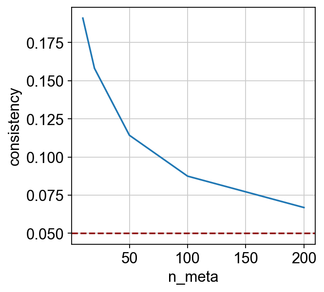
曲线越高,整合就越可靠。根据经验,如果曲线在0.05以上,就可以认为整合是可靠的。
应用模型——细胞和特征嵌入
(预计时间:约2分钟)
有了训练好的模型,可以使用 encode_data 函数对单细胞组学数据进行细胞嵌入。encode_data 的第一个参数指定了编码模态(之前的模态名之一),第二个参数指定了编码数据集。通常,我们将细胞嵌入存储在 obsm 中,名称为 "X_glue"。
[11]:
rna.obsm["X_glue"] = glue.encode_data("rna", rna)
atac.obsm["X_glue"] = glue.encode_data("atac", atac)
为了联合可视化两个组学层的细胞嵌入,我们构建了一个组合数据集。
[12]:
combined = ad.concat([rna, atac])
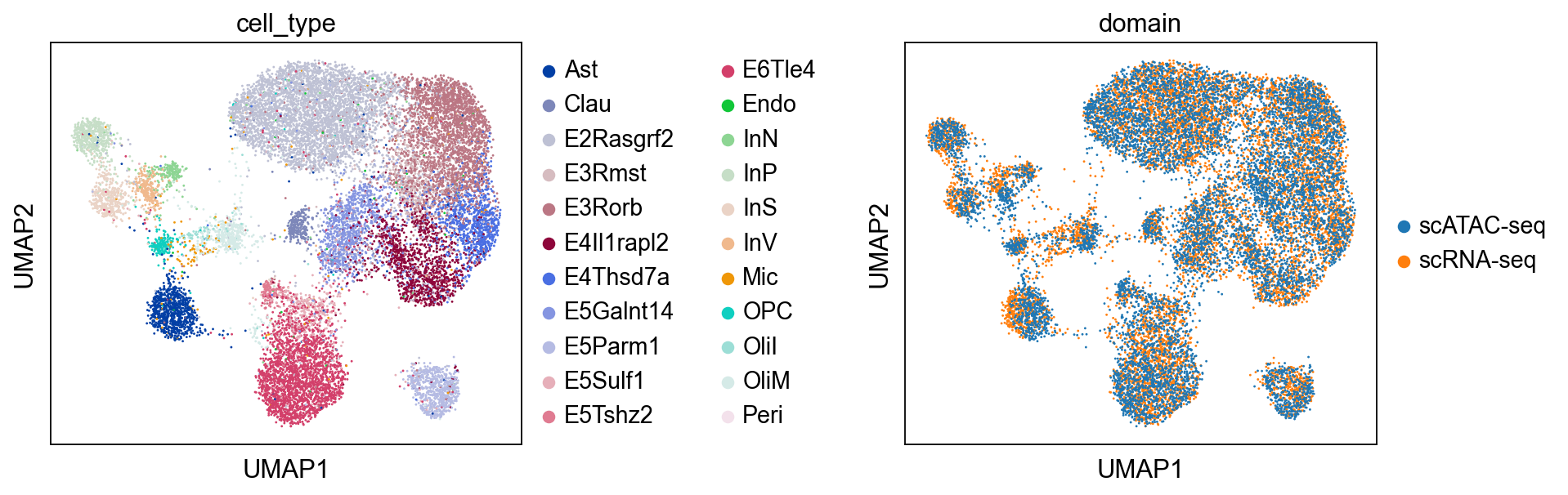
我们用UMAP来可视化对齐的嵌入。可以看到,两个组学层现在已经正确对齐了。
[13]:
sc.pp.neighbors(combined, use_rep="X_glue", metric="cosine")
sc.tl.umap(combined)
sc.pl.umap(combined, color=["cell_type", "domain"], wspace=0.65)
为了得到特征嵌入,可以使用 encode_graph 函数。
[14]:
feature_embeddings = glue.encode_graph(guidance_hvf)
feature_embeddings = pd.DataFrame(feature_embeddings, index=glue.vertices)
feature_embeddings.iloc[:5, :5]
[14]:
| 0 | 1 | 2 | 3 | 4 | |
|---|---|---|---|---|---|
| 0610009B22Rik | 0.003167 | 1.164528 | 0.001782 | 0.002524 | -0.001086 |
| 0610025J13Rik | 0.007353 | 1.800663 | -0.002449 | -0.001597 | 0.002197 |
| 1110002J07Rik | 0.001606 | 1.306113 | 0.002979 | -0.003802 | -0.002259 |
| 1110006O24Rik | 0.000742 | 1.436544 | 0.002607 | -0.005381 | -0.004283 |
| 1110020A21Rik | -0.003964 | 1.571156 | 0.006464 | 0.001598 | -0.000315 |
我们将特征嵌入存储在AnnData对象的 varm 中,名称也为 "X_glue"。
[15]:
rna.varm["X_glue"] = feature_embeddings.reindex(rna.var_names).to_numpy()
atac.varm["X_glue"] = feature_embeddings.reindex(atac.var_names).to_numpy()
我们现在保存带有细胞和特征嵌入的AnnData对象,以及仅包含高可变特征的引导图。
[16]:
rna.write("rna-emb.h5ad", compression="gzip")
atac.write("atac-emb.h5ad", compression="gzip")
nx.write_graphml(guidance_hvf, "guidance-hvf.graphml.gz")
关于使用GLUE嵌入进行调控推断的说明,请参考 第三步。