第三步:调控推断
在本教程中,我们将介绍如何使用GLUE特征嵌入来进行调控推断。我们继续使用之前的scRNA-seq和scATAC-seq数据集作为例子。
在这一例子中,我们将使用基于GLUE的调控推断来鉴定每个基因的显著顺式调控区(ATAC峰)。我们也将展示如何将额外的TF结合位点信息与基于GLUE鉴定的顺式调控区结合在一起构建的TF-靶基因调控图。
[1]:
import anndata as ad
import networkx as nx
import numpy as np
import pandas as pd
import scglue
import seaborn as sns
from IPython import display
from matplotlib import rcParams
from networkx.algorithms.bipartite import biadjacency_matrix
from networkx.drawing.nx_agraph import graphviz_layout
[2]:
scglue.plot.set_publication_params()
rcParams['figure.figsize'] = (4, 4)
读取中间结果
首先,读取 第二步 产生的包含细胞和特征嵌入的中间结果。
[3]:
rna = ad.read_h5ad("rna-emb.h5ad")
atac = ad.read_h5ad("atac-emb.h5ad")
guidance_hvf = nx.read_graphml("guidance-hvf.graphml.gz")
We will be using genomic coordinates a lot in BED format. It is convenient to store the variable names as a “name” column.
[4]:
rna.var["name"] = rna.var_names
atac.var["name"] = atac.var_names
由于GLUE模型是用高可变特征训练的,调控推断也只能在这些特征的范围内进行。因此,我们先将高可变特征提取出来,方便之后的使用。
[5]:
genes = rna.var.query("highly_variable").index
peaks = atac.var.query("highly_variable").index
用GLUE特征嵌入进行顺式调控推断
(预计时间:忽略不计)
我们首先将两个模态的特征索引和嵌入合并。
[6]:
features = pd.Index(np.concatenate([rna.var_names, atac.var_names]))
feature_embeddings = np.concatenate([rna.varm["X_glue"], atac.varm["X_glue"]])
We would also need to extract a “skeleton” graph on which to conduct regulatory inference. The “skeleton” serves to limit the search space of potential regulatory pairs, which helps reduce false positives caused by spurious correlations.
调控得分被定义为特征嵌入间的余弦相似度,余弦相似度是对称的,因此我们只选择RNA基因和ATAC峰之间的一个方向来避免重复计算。
自环也被忽略,因为目前的模型不能有意义地反应自调控。
[7]:
skeleton = guidance_hvf.edge_subgraph(
    e for e, attr in dict(guidance_hvf.edges).items()
    if attr["type"] == "fwd"
).copy()
调控推断可以使用 scglue.genomics.regulatory_inference 函数来进行,该函数接受特征索引和嵌入作为输入,并且使用上面生成的骨架图。
返回的对象也是一个图,具有以下额外的边属性:
"score":基因组特征间的调控得分,定义为特征嵌入间的余弦相似度;"pval":调控得分的*P*值,通过与随机打乱特征嵌入得到的调控得分NULL分布比较得到;"qval":调控得分的*Q*值,通过FDR修正*P*值得到。
[8]:
reginf = scglue.genomics.regulatory_inference(
    features, feature_embeddings,
    skeleton=skeleton, random_state=0
)
可以根据边属性(Q值 < 0.05)提取显著的调控关系。
[9]:
gene2peak = reginf.edge_subgraph(
    e for e, attr in dict(reginf.edges).items()
    if attr["qval"] < 0.05
)
可视化推断的顺式调控区域
(预计时间:忽略不计)
推断的顺式调控关系可以用 pyGenomeTracks 来可视化。你可以通过以下命令安装 pyGenomeTracks:
conda install -c bioconda pygenometracks
在画图之前,我们需要为 pygenometracks 命令准备输入文件。
Specifically, we save the ATAC peaks in BED format, and the inferred gene-peak connections in “links” format:
[10]:
scglue.genomics.Bed(atac.var).write_bed("peaks.bed", ncols=3)
scglue.genomics.write_links(
    gene2peak,
    scglue.genomics.Bed(rna.var).strand_specific_start_site(),
    scglue.genomics.Bed(atac.var),
    "gene2peak.links", keep_attrs=["score"]
)
接着准备一个轨道配置文件,如下所示(详细信息请参考他们的 文档):
[11]:
%%writefile tracks.ini

[Score]
file = gene2peak.links
title = Score
height = 2
color = YlGnBu
compact_arcs_level = 2
use_middle = True
file_type = links

[ATAC]
file = peaks.bed
title = ATAC
display = collapsed
border_color = none
labels = False
file_type = bed

[Genes]
file = gencode.vM25.chr_patch_hapl_scaff.annotation.gtf.gz
title = Genes
prefered_name = gene_name
height = 4
merge_transcripts = True
labels = True
max_labels = 100
all_labels_inside = True
style = UCSC
file_type = gtf

[x-axis]
fontsize = 12
Writing tracks.ini
最后,我们可以调用 pygenometracks 命令在一个合适的基因组范围内(例如*Gad2*基因周围区域)可视化推断的顺式调控关系:
[12]:
loc = rna.var.loc["Gad2"]
chrom = loc["chrom"]
chromLen = loc["chromEnd"] - loc["chromStart"]
chromStart = loc["chromStart"] - chromLen
chromEnd = loc["chromEnd"] + chromLen
!pyGenomeTracks --tracks tracks.ini \
    --region {chrom}:{chromStart}-{chromEnd} \
    --outFileName tracks.png 2> /dev/null
display.Image("tracks.png")
[12]:
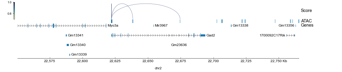
需要注意的是,在本教程中,指导图简单地使用了基因组重叠(请参考 第一步),所以推断的调控关系也仅限于近端启动子和基因本体区。
在实际的分析中,扩大基因组范围(例如,使用TSS上下游150kb随距离衰减加权)或者引入如Hi-C和eQTL的其他调控证据将是有益的(请参考我们的 案例研究)。
基于推断的顺式调控区域构建TF-靶基因调控网络
接着,我们将演示如何将GLUE推断的顺式调控区域与TF motif/ChIP-seq信息结合来构建TF-靶基因调控图。具体来说,我们采用的是 SCENIC pipeline,分为以下三个步骤:
使用
GRNBoost2生成一个共表达网络;结合顺式调控区域和TF motif/ChIP-seq数据生成顺式调控排序;
使用
cisTarget基于上述顺式调控排序修剪共表达网络。
如果要安装pyscenic,可以使用以下命令:
conda install -c conda-forge pyarrow cytoolz
pip install pyscenic
对于人和小鼠,第二步使用的TF motif/ChIP-seq数据可以从这里下载:
JASPAR motif结合:
http://download.gao-lab.org/GLUE/cisreg/JASPAR2022-hg19.bed.gz
http://download.gao-lab.org/GLUE/cisreg/JASPAR2022-hg38.bed.gz
http://download.gao-lab.org/GLUE/cisreg/JASPAR2022-mm9.bed.gz
http://download.gao-lab.org/GLUE/cisreg/JASPAR2022-mm10.bed.gz
ENCODE TF ChIP-seq:
http://download.gao-lab.org/GLUE/cisreg/ENCODE-TF-ChIP-hg38.bed.gz
http://download.gao-lab.org/GLUE/cisreg/ENCODE-TF-ChIP-hg19.bed.gz
http://download.gao-lab.org/GLUE/cisreg/ENCODE-TF-ChIP-mm10.bed.gz
http://download.gao-lab.org/GLUE/cisreg/ENCODE-TF-ChIP-mm9.bed.gz
原始调控推断流程参见 pySCENIC。
生成一个共表达网络
(预计时间:~5分钟)
首先,生成一个可用的TF列表,我们使用被scRNA-seq数据和TF motif/ChIP-seq数据同时覆盖的TF。
由于ENCODE ChIP-seq覆盖了非常少的小鼠TF,我们在本教程中将使用JASPAR motif结合数据:
[13]:
motif_bed = scglue.genomics.read_bed("JASPAR2022-mm10.bed.gz")
motif_bed.head()
[13]:
| chrom | chromStart | chromEnd | name | score | strand | thickStart | thickEnd | itemRgb | blockCount | blockSizes | blockStarts | |
|---|---|---|---|---|---|---|---|---|---|---|---|---|
| 0 | GL456210.1 | 159 | 171 | Zbtb6 | . | . | . | . | . | . | . | . |
| 1 | GL456210.1 | 242 | 253 | Osr2 | . | . | . | . | . | . | . | . |
| 2 | GL456210.1 | 266 | 278 | Pou2f3 | . | . | . | . | . | . | . | . |
| 3 | GL456210.1 | 505 | 517 | Eomes | . | . | . | . | . | . | . | . |
| 4 | GL456210.1 | 507 | 516 | Tbr1 | . | . | . | . | . | . | . | . |
[14]:
tfs = pd.Index(motif_bed["name"]).intersection(rna.var_names)
tfs.size
[14]:
532
由于pySCENIC CLI使用的是 loom 文件作为输入,我们需要将scRNA-seq数据保存为一个 loom 文件(只包含高可变基因和TF),我们也需要将TF列表保存为一个单独的 txt 文件。
[15]:
rna[:, np.union1d(genes, tfs)].write_loom("rna.loom")
np.savetxt("tfs.txt", tfs, fmt="%s")
The loom file will lack these fields:
{'X_umap', 'X_pca', 'X_glue', 'PCs'}
Use write_obsm_varm=True to export multi-dimensional annotations
使用命令 pyscenic grn 来生成一个共表达网络。
[16]:
!pyscenic grn rna.loom tfs.txt \
    -o draft_grn.csv --seed 0 --num_workers 20 \
    --cell_id_attribute cells --gene_attribute genes
2022-08-12 12:30:12,903 - pyscenic.cli.pyscenic - INFO - Loading expression matrix.

2022-08-12 12:30:13,236 - pyscenic.cli.pyscenic - INFO - Inferring regulatory networks.
Numba: Attempted to fork from a non-main thread, the TBB library may be in an invalid state in the child process.
Numba: Attempted to fork from a non-main thread, the TBB library may be in an invalid state in the child process.
Numba: Attempted to fork from a non-main thread, the TBB library may be in an invalid state in the child process.
Numba: Attempted to fork from a non-main thread, the TBB library may be in an invalid state in the child process.
Numba: Attempted to fork from a non-main thread, the TBB library may be in an invalid state in the child process.
Numba: Attempted to fork from a non-main thread, the TBB library may be in an invalid state in the child process.
Numba: Attempted to fork from a non-main thread, the TBB library may be in an invalid state in the child process.
Numba: Attempted to fork from a non-main thread, the TBB library may be in an invalid state in the child process.
Numba: Attempted to fork from a non-main thread, the TBB library may be in an invalid state in the child process.
Numba: Attempted to fork from a non-main thread, the TBB library may be in an invalid state in the child process.
Numba: Attempted to fork from a non-main thread, the TBB library may be in an invalid state in the child process.
Numba: Attempted to fork from a non-main thread, the TBB library may be in an invalid state in the child process.
Numba: Attempted to fork from a non-main thread, the TBB library may be in an invalid state in the child process.
Numba: Attempted to fork from a non-main thread, the TBB library may be in an invalid state in the child process.
Numba: Attempted to fork from a non-main thread, the TBB library may be in an invalid state in the child process.
Numba: Attempted to fork from a non-main thread, the TBB library may be in an invalid state in the child process.
Numba: Attempted to fork from a non-main thread, the TBB library may be in an invalid state in the child process.
Numba: Attempted to fork from a non-main thread, the TBB library may be in an invalid state in the child process.
Numba: Attempted to fork from a non-main thread, the TBB library may be in an invalid state in the child process.
Numba: Attempted to fork from a non-main thread, the TBB library may be in an invalid state in the child process.
Numba: Attempted to fork from a non-main thread, the TBB library may be in an invalid state in the child process.
preparing dask client
parsing input
creating dask graph
20 partitions
computing dask graph
not shutting down client, client was created externally
finished

2022-08-12 12:34:03,906 - pyscenic.cli.pyscenic - INFO - Writing results to file.
经由ATAC峰生成TF顺式调控排序
(预计时间:~1小时)
我们使用 scglue.genomics.window_graph 函数扫描基因组来连接ATAC峰与TF motif结合位点,这将需要一些时间(~1小时)。
[17]:
peak_bed = scglue.genomics.Bed(atac.var.loc[peaks])
peak2tf = scglue.genomics.window_graph(peak_bed, motif_bed, 0, right_sorted=True)
peak2tf = peak2tf.edge_subgraph(e for e in peak2tf.edges if e[1] in tfs)
根据GLUE推断的gene-peak连接和motif支持的peak-TF连接,ATAC峰可以作为一个桥梁帮助推断gene-TF连接。
我们可以使用 scglue.genomics.cis_regulatory_ranking 函数来将gene-peak和peak-TF连接合并为一个gene-TF顺式调控排序。由于每个基因可以连接到不同数量、长度的ATAC峰,合并的基因-TF连接不是直接可比的。因此,该函数将观察到的连接与(根据峰长度分层)随机采样的连接进行比较,以评估其富集程度,然后用于排序每个TF的调控基因。
[18]:
gene2tf_rank_glue = scglue.genomics.cis_regulatory_ranking(
    gene2peak, peak2tf, genes, peaks, tfs,
    region_lens=atac.var.loc[peaks, "chromEnd"] - atac.var.loc[peaks, "chromStart"],
    random_state=0
)
gene2tf_rank_glue.iloc[:5, :5]
/rd2/user/caozj/GLUE/conda/lib/python3.8/site-packages/scglue/genomics.py:724: FutureWarning: biadjacency_matrix will return a scipy.sparse array instead of a matrix in NetworkX 3.0
  gene2region = biadjacency_matrix(gene2region, genes, regions, dtype=np.int16, weight=None)
/rd2/user/caozj/GLUE/conda/lib/python3.8/site-packages/scglue/genomics.py:725: FutureWarning: biadjacency_matrix will return a scipy.sparse array instead of a matrix in NetworkX 3.0
  region2tf = biadjacency_matrix(region2tf, regions, tfs, dtype=np.int16, weight=None)
[18]:
| Zbtb6 | Osr2 | Pou2f3 | Eomes | Tbr1 | |
|---|---|---|---|---|---|
| genes | |||||
| 0610009B22Rik | 1193.5 | 1211.0 | 1155.5 | 1115.5 | 1098.5 |
| 1110002J07Rik | 1193.5 | 1211.0 | 1155.5 | 1115.5 | 1098.5 |
| 1110006O24Rik | 1193.5 | 1211.0 | 1155.5 | 1115.5 | 1098.5 |
| 1110020A21Rik | 1193.5 | 1211.0 | 1155.5 | 1115.5 | 1098.5 |
| 1110060G06Rik | 1193.5 | 1211.0 | 1155.5 | 1115.5 | 1098.5 |
经由近端启动子生成TF顺式调控排序(可选)
(预计时间:~1小时)
上述方法的一个潜在的限制是,若某基因没有与调控ATAC峰相连,将被丢掉。作为补充,我们也可以使用TSS周围的近端启动子区域来生成顺式调控排序,与原始pySCENIC流程相同。
我们再次使用 scglue.genomics.window_graph 函数扫描基因组来连接TSS周围的近端启动子区域(-500到+500bp)与TF motif结合位点,在结果图中近端启动子区域的命名与相应基因一致。
[19]:
flank_bed = scglue.genomics.Bed(rna.var.loc[genes]).strand_specific_start_site().expand(500, 500)
flank2tf = scglue.genomics.window_graph(flank_bed, motif_bed, 0, right_sorted=True)
与上一章节相同,我们使用 scglue.genomics.cis_regulatory_ranking 函数来生成一个补充的顺式调控排序,与之前的排序有如下的差异:
基因-峰连接被替换为基因-近端启动子连接,因为每个TSS周围的近端启动子区域与其对应的基因具有相同的名称,所以基因-近端启动子连接图就是一个自环图;
由于每个基因有且仅有一个长度相同的近端启动子区域,因此无需通过分层随机抽样评估TF富集,我们将
n_samples设为0以跳过采样过程。
[20]:
gene2flank = nx.Graph([(g, g) for g in genes])
gene2tf_rank_supp = scglue.genomics.cis_regulatory_ranking(
    gene2flank, flank2tf, genes, genes, tfs,
    n_samples=0
)
gene2tf_rank_supp.iloc[:5, :5]
/rd2/user/caozj/GLUE/conda/lib/python3.8/site-packages/scglue/genomics.py:724: FutureWarning: biadjacency_matrix will return a scipy.sparse array instead of a matrix in NetworkX 3.0
  gene2region = biadjacency_matrix(gene2region, genes, regions, dtype=np.int16, weight=None)
/rd2/user/caozj/GLUE/conda/lib/python3.8/site-packages/scglue/genomics.py:725: FutureWarning: biadjacency_matrix will return a scipy.sparse array instead of a matrix in NetworkX 3.0
  region2tf = biadjacency_matrix(region2tf, regions, tfs, dtype=np.int16, weight=None)
[20]:
| Zbtb6 | Osr2 | Pou2f3 | Eomes | Tbr1 | |
|---|---|---|---|---|---|
| genes | |||||
| 0610009B22Rik | 1087.5 | 1053.5 | 1026.0 | 1016.5 | 1018.5 |
| 1110002J07Rik | 1087.5 | 1053.5 | 1026.0 | 1016.5 | 1018.5 |
| 1110006O24Rik | 1087.5 | 1053.5 | 1026.0 | 1016.5 | 1018.5 |
| 1110020A21Rik | 1087.5 | 1053.5 | 1026.0 | 1016.5 | 1018.5 |
| 1110060G06Rik | 1087.5 | 1053.5 | 1026.0 | 1016.5 | 1018.5 |
使用顺式调控排序修剪共表达网络
(预计时间:~5分钟)
最后一步,我们将使用上述顺式调控排序修剪共表达网络来保留的存在顺式调控证据的TF-基因连接。为此,我们需要准备以下文件:
一个或多个包含顺式调控排序的
feather文件;一个将顺式调控排序文件中的列名映射到TF名的
tsv注释文件。
这里我们有两个不同的顺式调控排序(基于ATAC的和基于启动子的),它们的列名相同,我们需要把它们根据信息来源进行区分。
[21]:
gene2tf_rank_glue.columns = gene2tf_rank_glue.columns + "_glue"
gene2tf_rank_supp.columns = gene2tf_rank_supp.columns + "_supp"
我们可以使用 scglue.genomics.write_scenic_feather 函数将顺式调控排序保存为与兼容 pySCENIC 兼容的 feather 文件。
[22]:
scglue.genomics.write_scenic_feather(gene2tf_rank_glue, "glue.genes_vs_tracks.rankings.feather")
scglue.genomics.write_scenic_feather(gene2tf_rank_supp, "supp.genes_vs_tracks.rankings.feather")
然后使用以下格式的注释文件:
[23]:
pd.concat([
    pd.DataFrame({
        "#motif_id": tfs + "_glue",
        "gene_name": tfs
    }),
    pd.DataFrame({
        "#motif_id": tfs + "_supp",
        "gene_name": tfs
    })
]).assign(
    motif_similarity_qvalue=0.0,
    orthologous_identity=1.0,
    description="placeholder"
).to_csv("ctx_annotation.tsv", sep="\t", index=False)
我们现在可以使用pySCENIC命令 pyscenic ctx 来修剪共表达网络(这里 rank_threshold 根据高可变基因的数量等比缩小):
[24]:
!pyscenic ctx draft_grn.csv \
    glue.genes_vs_tracks.rankings.feather \
    supp.genes_vs_tracks.rankings.feather \
    --annotations_fname ctx_annotation.tsv \
    --expression_mtx_fname rna.loom \
    --output pruned_grn.csv \
    --rank_threshold 500 --min_genes 1 \
    --num_workers 20 \
    --cell_id_attribute cells --gene_attribute genes 2> /dev/null
[########################################] | 100% Completed | 35.40 s
得到修剪后的网络可以使用 scglue.genomics.read_ctx_grn 函数读取为一个networkx图:
[25]:
grn = scglue.genomics.read_ctx_grn("pruned_grn.csv")
可视化推断得到的TF-靶基因网络
(预计时间:忽略不计)
TF-靶基因网络可以直接使用networkx来可视化:
[26]:
rcParams['figure.figsize'] = (10, 10)
nx.draw(grn, graphviz_layout(grn), with_labels=True)
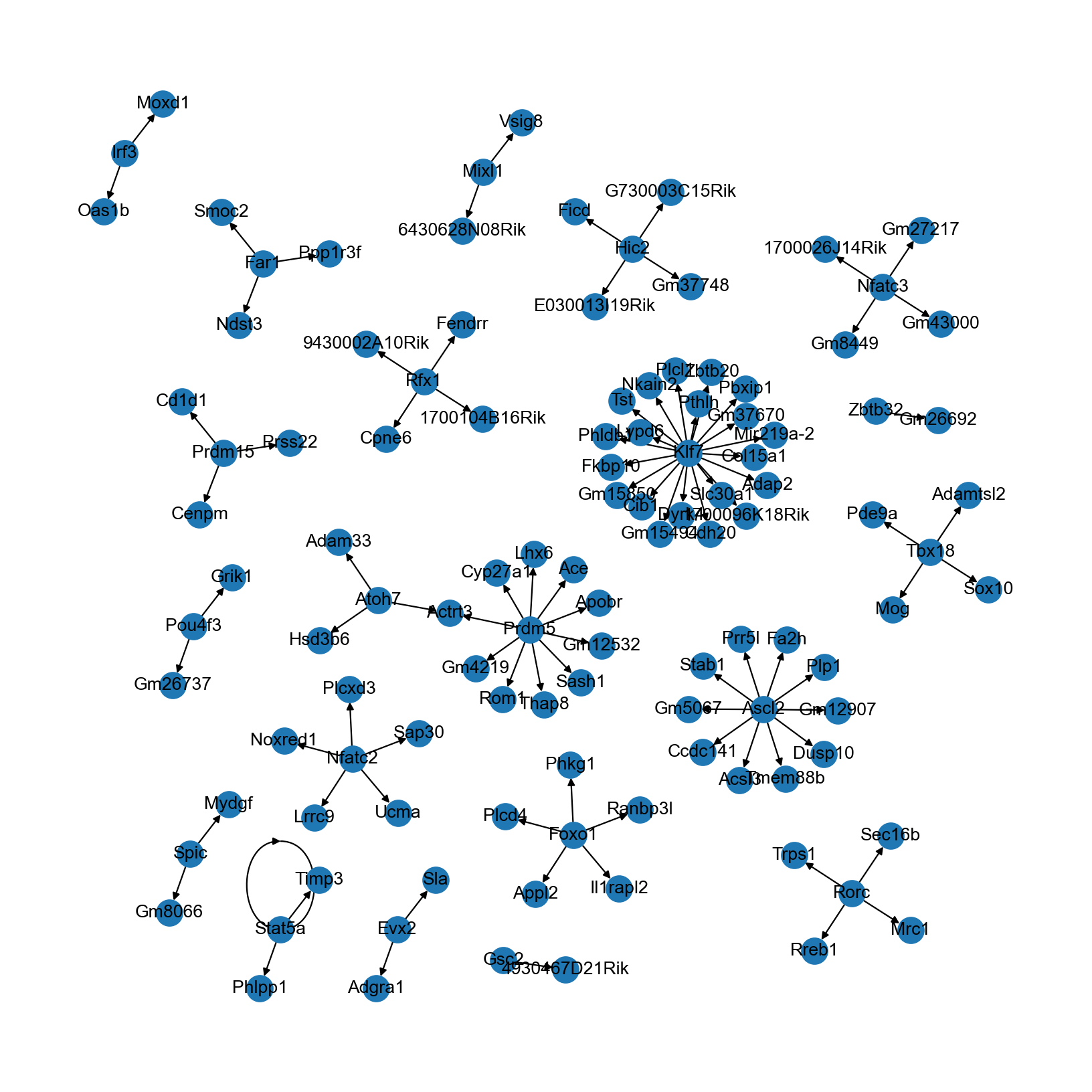
您也可以将此图(比如以 graphml 格式)导出到诸如 Cytoscape 和 Gephi 等其他软件以进行更多的自定义调整。
[27]:
nx.write_graphml(grn, "pruned_grn.graphml.gz")
需要说明的是,这里推断得到的网络具有较少的节点数和连通性。在真实的数据分析中,我们建议:
在构建引导图时扩展基因组范围(比如TSS上下游150kb内距离衰减加权),并引入像Hi-C和eQTL这样的额外调控证据(参见我们的 案例研究);
增加高可变基因数(比如增加到4000或6000)以将更多基因纳入到分析当中。